LVPS Positioning Algorithm
This algorithm is an original creative work I developed in 2023 over the course of several months and many iterations.

No generative A.I. was used to assist in the design or development of the algorithm. The algorithm does, however, make use of various A.I. techniques, including vision recognition and a customized genetic algorithm.
Summary
Going from a map and some images to a set of coordinates and heading is quite a task. Several math and computer science techniques are combined to produce a reasonable position estimate, and the process is described on this page.

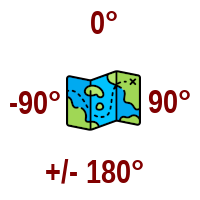
It is important to note that within the context of LVPS, I define 0° as directly in front of the vehicle, -90° represents port (left) side, and 90° represents the starboard (right) side of the vehicle. -180° or 180° both represent the rear of the vehicle. Click the flow chart to see a visual representation of the full algorithm.
Vehicle-Relative Heading

Map-Relative Heading
Detecting Landmarks

On the map, some known landmarks are identified. The known/mapped information for each landmark includes:
Known Coordinates - [X,Y]
Size - I use mm, but it could be anything as long as it’s consistent
Pattern - If using IR lights (square, triangle, vertical line, etc)
TFLite Model - trained for this object’s detection (multiple models can be used simultaneously)
Name/ID - within the Model
There may be as few as 2 landmarks, or many more. The coordinates given to these landmarks are the basis of all coordinates for the plane.
Landmarks can be outside the map boundaries, within, or any combination.
There is slightly different landmark detection logic for different model types, but the base class for landmark detection can be found here.
Smoothing

The values returned by our object detection models can be a little erratic. When an object first appears in the view (after some movement), it can take a few frames for the bounding box to narrow down as far as it's going to. We want the best bounding boxes we can get.
The process is a little more complicated than what’s shown below, but this is the essence of it:
Smoothing Technique Summary
The object detection is repeated a given number of times until we have a nice set of samples.
From that set of samples, we find means and standard deviations for the different bounding boxes.
We drop any obvious outliers.
The mean of the remaining values becomes what we actually consider to be the landmark's bounding box.
Mathematical Notation

I am not a mathematician, so my symbols and notations may differ from norms, but I had to choose some. For purposes of describing the calculations, I will use the following notation:
↑ A ray from the front of the vehicle, or 0°, or on diagrams, I may not this as a ray named Z (for zero).
∠↑ LA Angle between 0° and where LA visually appears. If you draw a ray from the vehicle center to LA, this represents the angle between ↑ and the LA ray you just imagined.
※ Represents the current X,Y coordinates of the center of the vehicle.
Calculating Direction

Once we have identified landmarks, which camera they each showed up on, and the pixel boundaries of each object, we can use that to find the angle of the center of each landmark, relative to the front of the vehicle.
Then, we will end up with knowledge of things like Landmark A is at 90° and Landmark B is at -90°. As long as our vehicle is not upside down, that tells us we are directly between the two landmarks.
Of course, it's rarely going to be that simple. The diagram below shows the horizontal angles involved in the calculations we will need to do. To read through the code for this, a good place to start is the extract_object_view_angles method of the PositionEstimator class.

Starting with Landmark A, we want to find the position in degrees, where it appears visually, relative to the front of the vehicle (↑).
Using boundary boxes given by the vision model(s), convert the pixel center of each landmark to degrees from horizontal field of view center, with 0° being the horizontal center. I'm going to spare the details of how I do that for now, but it's not that complicated.
Find the angle between ↑ and C1 (the camera horizontal focal center). This tells us at what degrees the camera is currently aimed.
Find the angle between C1 and LA. This tells us how far landmark A appears to be from the center of camera 1. That is going to be the angle between ↑ and C1 (the camera horizontal focal center).
Finding difference between the angles found in step 2 and 3 will provide us with visual horizontal position (in degrees) of the landmark, relative to the front of the vehicle (↑).
We repeat the steps above for every landmark and every camera. In addition to keeping the camera where the landmark was found, the pixel location, and the relative position (in degrees), we also store a confidence value, which was provided by the vision model. If a landmark shows up twice (maybe the same camera saw it twice when rotation was smaller than the FOV), only the version with the highest confidence is used for future calculations.
Calculating Distance

The best we can do, given only visually observable information with imprecise bounding boxes, is use a few trig calculations to estimate distances. The following diagram shows the angles we have to work with.
In this case, I have used a series of vertically-aligned IR lights as an example of a landmark. So, object detection should have done a pretty decent job of identifying the boundaries for this.
The code for this starts in the To read through the code for this, a good place to start is the extract_distances method of the PositionEstimator class.

We also have to take altitude into account. If the cameras are positioned higher or lower than the landmark, the landmark will appear shorter than if it were being observed with its center at camera level.
To illustrate, lets assume the camera is at a higher altitude than the landmark. In this case, we can project (imagine) a right triangle overlaying the view above, with the 90° angle vertically above the landmark. One of the legs is the projection "top", PT (currently unknown). The hypotenuse, LB, is the segment between the camera and the landmark bottom. We use a second oblique triangle, with sides being LB (landmark bottom), LT (landmark top), and LH (landmark height).

In the diagram, PT is the projection "top", and that is the value we are solving for. It represents the ground distance between the camera and the landmark.
Beginning with the oblique triangle...
Calculate ∠ LH , or the visual height, in degrees, of the landmark. I need to add a section on how that is done, but we basically use knowledge of the image resolution, the resolution of the down-scaled copy we fed to the object detection model, the current vertical field of view of the camera, and the boundary box height of the landmark.
Find the degree/height ratio in our current view of the landmark. By this, I mean how many degrees per inch, mm, or whatever unit the height is mapped in.
Use the degree/height ratio to calculate how many degrees were added to the visual height of the landmark, when we overlaid the projection. In the diagram, this is highlighted by the green dashed arc. It is the visual height (degrees) of the projection extension, if we were able to observe it.
Find the visual projection height ∠ PH (in degrees) by adding the visual degree height of the landmark to the projection extension degree height, and we now have a second angle in our right triangle (identified by the blue dashed arc).
Now back to the right triangle...
Calculate the projection height PH (camera altitude - landmark bottom) in units, not degrees. We know these values because altitude is available on the vehicle any time, and the unit height of the landmark is available by consulting the map.
Find the hypotenuse: LB = PH / sin(∠ PH )
Finally find our ground distance, PT = √( LB ² - PH ²)
“Fuzzy” Trig
As I said, I’m not a mathematician and I’m probably really stepping in it here. I couldn’t find any established math techniques for doing exactly what need (which I’m calling “fuzzy” trig), so I just made up my own.
After repeating the calculations above for every landmark found on every camera at one point in time, we have a lot of measurements, with varying degrees of accuracy. Any distances between two landmarks are known facts, based on our predefined map, which has concrete X,Y values for each landmark.

Assuming the camera mounts have not been damaged, we can have high confidence in the vehicle-relative angle of each landmark (relative to the front of the vehicle), as reported by the object detection models. However, the vehicle-to-landmark distance measurements are estimates, based only on vision, which is a problem.
Let's assume we have found two landmarks, which we will call LA and LB. Let's also assume the object detection model did correctly identify these landmarks (which isn't an entirely safe assumption, but we'll ignore that for now)
Focusing on just that pair of sighted landmarks, we can observe and calculate the visual degrees ∠ LALB between the two (from the vehicle's perspective) using the known field of view, etc. In the diagram below, that angle is shown with the red arc. The other known, segment LALB, has a length of the distance between the two landmarks.
LIDAR

In another pass at collecting data (if configured), LIDAR-based measurement is attempted, for each landmark where that is possible.
A system configuration determines whether this LIDAR pass happens. Additionally, each landmark defined in the map has a setting indicating whether the landmark should be visible to LIDAR. If so, the second pass checks the LIDAR data at the horizontal angle believed to currently contain the landmark (within .5 degrees either direction).
If we get a LIDAR hit that seems reasonable, we substitute it for the visual-based distance, and boost the confidence value of that distance measurement (which will shrink the search space on that particular value when the Genetic Length Finder algorithm takes over.
Genetic Length Finder

Given that every vehicle-to-landmark measurement is either visually estimated or returned from LIDAR that has about a 2% margin of error, it is almost certain that if we try to triangulate with the measurements above, no triangle will match. So, we need to focus on the estimated lengths, and play with them a little bit until we come up with some workable values.
To accomplish this, I created a genetic length finder, which uses an evolutionary algorithm to find potential improvements to the estimated distances. I will probably add another section on that later, but the technique is summarized very well in Grokking Artificial Intelligence Algorithms (Hurbans), as well as various other sources.

Essentially it repeatedly tries different potential values by 'mating' solution sets, finding the best performing ones and culling the low performers, until some condition is met (time limit, good enough solutions found, etc).
I won't go much more into detail beyond that, except to say that search algorithm is coded in such a way that lower confidence values (visually-estimated distances) are allowed more room to 'explore' than higher confidence values (LIDAR). There is a lot to discuss there, but it needs a dedicated page with some code samples to adequately explain.

This search has to happen for each estimated distance. So, if there are a lot of visible landmarks, this can become a performance bottleneck. To improve performance, the code can do up to 3 of the searches simultaneously on different cores (both Nvidia Nano and Pi CM4 have only 4 cores, so I limit that to 3 for now).
There is a lot of room for performance improvement in this particular area. While the genetic search algorithm does seem to work pretty well, it is very expensive, time-wise. A faster solution may be possible by making use of the Fuzzy Circle techniques (Anand & Bharatraj). For now, I will leave that as a future optimization.
Extracting Coordinates & Heading

The length search algorithm will return many potential candidates for each vehicle-to-landmark distance. From each returned, we convert angles to slope, and use geometry to plot an X,Y coordinate. Then we try to determine if that position is even possible.
The set of possibilities will include coordinates for where we are upside down and right-side up. We are only dealing with ground-dwelling vehicles at this point, so I throw out all coordinates where the two landmarks appear on the wrong sides.
The map also has a fantastic hint. The map has boundaries of its own. Each coordinate pair is matched up against those boundaries, and if it is too far out of bounds (according to a configured threshold), that coordinate pair also gets thrown out.
After all of that, we are left with some possible coordinates that hopefully look quite similar.
Clustering

In order to further narrow down and improve the coordinates before coming up with a final decision, we apply K-Means Clustering, in two passes. The Scikit Learn package is used to accomplish this.
One pass calculates what the map-relative heading (remember, 0° means north in my coordinate system) for each potential potential position. We look at the mean/standard deviation among the headings, and if there is significant variance, we generate two clusters, based on heading, and choose the cluster that is densest (meaning it has the least heading variation among its headings).
If we have done heading clustering, the less dense set of coordinates is thrown out. On the second pass, assuming we still have enough potential coordinates to look for density, we again check the mean and standard deviation to see if there is significant variance, this time we use distance from (0,0) as the metric.
As before, if clustering is triggered, we divide into two groups using K-Means, and remove the set that has the least density.
Final Coordinate Selection

After clustering is applied, we are left with a significantly smaller set of potential coordinate values (sometimes none). Whatever is left, we find the centroid X,Y coordinate, and calculate what the heading would be, if the vehicle was sitting in that position.
The centroid X, centroid Y, calculated heading, plus a calculated confidence value are returned as the final result.
The final product of this algorithm is an [ X, Y] coordinate, corresponding to the map, a heading in degrees, and a confidence indicator.
The confidence value is calculated based on things like how many LIDAR hits we received, how many landmarks were found, and other criteria.
If the vehicle / device is not satisfied with the confidence value, it can adjust its position slightly and re-run the algorithm.
References
Hurbans R. (2020). Evolutionary Algorithms. In R. Hurbans, Grokking Artificial Intelligence Algorithms (pp. 91-135). Manning.
Anand C.J. & Bharatraj, J. (2018). Gaussian Qualitative Trigonometric Functions in a Fuzzy Circle. Hindawi, 10.1155/2018/8623465. https://doi.org/10.1155/2018/8623465
K-means Clustering. (n.d.). In Wikipedia. Retrieved November 4, 2023, from https://en.wikipedia.org/wiki/K-means_clustering